3D Subduction from Schellart et al, 2010
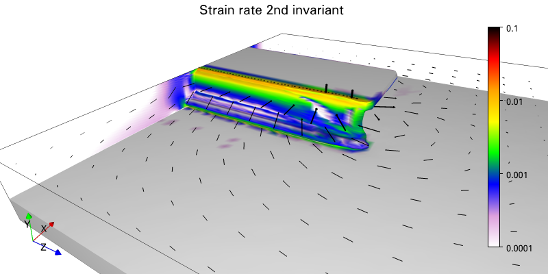
This notebook reproduces a three-dimensional 7,000 km wide subducting plate as shown in Figure S3c of Schellart et al, 2010.
References
- Schellart, W. P. and Stegman, D. R. and Farrington, R. J. and Freeman, J. and Moresi, L. Cenozoic Tectonics of Western North America Controlled by Evolving Width of Farallon Slab. Science, 16 July 2010, Vol. 329, Issue 5989, pp. 316-319 Schelart et al, 2010.
In [1]:
import underworld as uw
import math
from underworld import function as fn
import glucifer
import numpy as np
import os
In [2]:
outputPath = os.path.join(os.path.abspath("."),"output/")

if uw.rank()==0:
    if not os.path.exists(outputPath):
        os.makedirs(outputPath)
uw.barrier()
Setup parameters
In [3]:
# slab width
slabWidth      = 3.5 # 1e3 km

yRes = 8  # use yRes=48 to reproduce results
xRes = yRes*3
zRes = yRes*3
dim  = 3
boxLength = 7.0  # 1e3 km
boxHeight = 1.0  # 1e3 km
boxWidth  = 7.0  # 1e3 km
Create mesh and finite element variables
In [4]:
mesh = uw.mesh.FeMesh_Cartesian( elementType = ("Q1/dQ0"),
                                 elementRes  = (xRes, yRes, zRes),
                                 minCoord    = (0., 0., 0.),
                                 maxCoord    = (boxLength, boxHeight, boxWidth))

velocityField  = uw.mesh.MeshVariable( mesh=mesh,         nodeDofCount=dim )
pressureField  = uw.mesh.MeshVariable( mesh=mesh.subMesh, nodeDofCount=1 )
In [5]:
# set initial conditions (and boundary values)
velocityField.data[:] = [0.,0.,0.]
pressureField.data[:] = 0.
If reloading from checkpointing, load these files
In [6]:
# ## load mesh, velocity, pressure, temperature & temperatureDot fields via checkpoint files
# step = 1
# mesh.load(               outputPath+'mesh.'+                str(step).zfill(5) +'.h5')
# velocityField.load(      outputPath+'velocityField.'+       str(step).zfill(5) +'.h5')
# pressureField.load(      outputPath+'pressureField.'+       str(step).zfill(5) +'.h5')
Create the particle swarm
In [7]:
swarm       = uw.swarm.Swarm( mesh=mesh )
materialIndex   = swarm.add_variable( dataType="int", count=1 )
# create tracer swarms
trenchSwarm = uw.swarm.Swarm( mesh=mesh )
slab1Swarm  = uw.swarm.Swarm( mesh=mesh )
slab2Swarm  = uw.swarm.Swarm( mesh=mesh )
slab3Swarm  = uw.swarm.Swarm( mesh=mesh )
If reloading from checkpointing, load these files
In [8]:
# # load swarm, materialVariable and viscosityVariable from checkpoint
# swarm.load(         outputPath +'swarm.'            + str(step).zfill(5) +'.h5')
# materialIndex.load( outputPath +'materialIndex.' + str(step).zfill(5) +'.h5')

# trenchSwarm.load(   outputPath +'trenchSwarm.'      + str(step).zfill(5) +'.h5')
# slab1Swarm.load(    outputPath +'slab1Swarm.'       + str(step).zfill(5) +'.h5')
# slab2Swarm.load(    outputPath +'slab2Swarm.'       + str(step).zfill(5) +'.h5')
# slab3Swarm.load(    outputPath +'slab3Swarm.'       + str(step).zfill(5) +'.h5')
else, layout swarm & tracer swarm
In [9]:
swarmLayout = uw.swarm.layouts.GlobalSpaceFillerLayout( swarm=swarm, particlesPerCell=20 )
swarm.populate_using_layout( layout=swarmLayout )

# add tracer particles
tracerSwarmRes = 51


# add particles to tracer swarms
# trench
particleCoord = np.zeros((tracerSwarmRes,3))
particleCoord[:,0] = 3.5
particleCoord[:,1] = 1.0
particleCoord[:,2] = np.linspace(0, slabWidth, tracerSwarmRes)
temp = trenchSwarm.add_particles_with_coordinates(particleCoord)

# slab midplane, z = 0
particleCoord = np.zeros((tracerSwarmRes,3))
particleCoord[:,0] = np.linspace(3.5, 5.7, tracerSwarmRes)
particleCoord[:,1] = 0.95
particleCoord[:,2] = 0.0
temp = slab1Swarm.add_particles_with_coordinates(particleCoord)

# slab midplane, z = 1.5
particleCoord[:,2] = 1.5
temp = slab2Swarm.add_particles_with_coordinates(particleCoord)

# slab midplane, z = 3.0
particleCoord[:,2] = 2.99
temp = slab3Swarm.add_particles_with_coordinates(particleCoord)
Allocate materials to particles
In [10]:
# initialise the 'materialVariable' data to represent two different materials.
upperMantleIndex = 0
lowerMantleIndex = 1
upperSlabIndex   = 2
core1SlabIndex   = 3
core2SlabIndex   = 4
lowerSlabIndex   = 5
In [11]:
# Initial material layout has a flat lying slab with at 15\degree perturbation
lowerMantleY   = 0.35
slabUpperShape = np.array([ (3.5,1.000 ), (5.7,1.000 ), (5.7,0.975), (3.5,0.975), (3.32,0.900), (3.32,0.925) ])
slabCore1Shape = np.array([ (3.5,0.975 ), (5.7,0.975 ), (5.7,0.950), (3.5,0.950), (3.32,0.875), (3.32,0.900) ])
slabCore2Shape = np.array([ (3.5,0.950 ), (5.7,0.950 ), (5.7,0.925), (3.5,0.925), (3.32,0.850), (3.32,0.875) ])
slabLowerShape = np.array([ (3.5,0.925 ), (5.7,0.925 ), (5.7,0.900), (3.5,0.900), (3.32,0.825), (3.32,0.850) ])

slabUpper = fn.shape.Polygon( slabUpperShape )
slab1Core = fn.shape.Polygon( slabCore1Shape )
slab2Core = fn.shape.Polygon( slabCore2Shape )
slabLower = fn.shape.Polygon( slabLowerShape )

# initialise everying to be upper mantle material
materialIndex.data[:] = upperMantleIndex

# change matieral index if the particle is not upper mantle
for index in range( len(swarm.particleCoordinates.data) ):
    coord = swarm.particleCoordinates.data[index][:]
    if coord[1] < lowerMantleY:
        materialIndex.data[index]     = lowerMantleIndex
    if coord[2] < slabWidth:
        if slabUpper.evaluate(tuple(coord)):
            materialIndex.data[index] = upperSlabIndex
        if slab1Core.evaluate(tuple(coord)):
            materialIndex.data[index] = core1SlabIndex
        if slab2Core.evaluate(tuple(coord)):
            materialIndex.data[index] = core2SlabIndex
        if slabLower.evaluate(tuple(coord)):
            materialIndex.data[index] = lowerSlabIndex
Plot the initial material layout
In [12]:
#First project material index on to mesh for use in plotting material isosurfaces
materialField     = uw.mesh.MeshVariable( mesh, 1 )
materialProjector = uw.utils.MeshVariable_Projection( materialField, materialIndex, type=0 )
materialProjector.solve()
In [13]:
# plot isosurface for materialField values = 0.5
figMaterialLayout = glucifer.Figure( figsize=(1000,400), quality=2, title='Material Index', axis=True )
figMaterialLayout.append(glucifer.objects.IsoSurface( mesh, materialField, isovalues=[0.5],
                                                     isowalls=True, shift=1, discrete=True))
figMaterialLayout.append(glucifer.objects.Points(trenchSwarm, colourBar=False, pointSize=2 ))
figMaterialLayout.append(glucifer.objects.Points(slab1Swarm,  colourBar=False, pointSize=2 ))
figMaterialLayout.append(glucifer.objects.Points(slab2Swarm,  colourBar=False, pointSize=2 ))
figMaterialLayout.append(glucifer.objects.Points(slab3Swarm,  colourBar=False, pointSize=2 ))

camera = ['rotate y 60', 'rotate x 30']
figMaterialLayout.script(camera)
figMaterialLayout.show()

Set up material parameters and functions
In [14]:
upperMantleViscosity =    1.0
lowerMantleViscosity =  100.0
upperViscosity       = 1000.0
core1Viscosity       =  300.0
core2Viscosity       =   50.0
lowerViscosity       =  200.0

# The yeilding of the upper slab is dependent on the strain rate.
strainRate_2ndInvariant = fn.tensor.second_invariant(
                            fn.tensor.symmetric(
                            velocityField.fn_gradient ))
cohesion = 0.06
vonMises = 0.5 * cohesion / (strainRate_2ndInvariant+1.0e-18)

# The upper slab viscosity is the minimum of the 'slabViscosity' or the 'vonMises'
slabYieldvisc = fn.exception.SafeMaths( fn.misc.min(vonMises, upperViscosity) )

# Viscosity function for the materials
viscosityMap = { upperMantleIndex : upperMantleViscosity,
                 lowerMantleIndex : lowerMantleViscosity,
                 upperSlabIndex   : slabYieldvisc,
                 core1SlabIndex   : core1Viscosity,
                 core2SlabIndex   : core2Viscosity,
                 lowerSlabIndex   : slabYieldvisc,
               }
viscosityFn = fn.branching.map( fn_key = materialIndex, mapping = viscosityMap )
In [15]:
viscosityField = uw.mesh.MeshVariable( mesh, 1 )
viscosityProjector = uw.utils.MeshVariable_Projection( viscosityField, viscosityFn, type=0 )
viscosityProjector.solve()
In [16]:
viscosity = glucifer.objects.Surface( mesh, viscosityField, crossSection="z 0%", logScale=True, axis=True  )
viscosity.colourBar["tickvalues"] = [1, 10, 100, 1000]

figViscosity = glucifer.Figure( figsize=(1000,300), quality=2, title='Viscosity Field' )
figViscosity.append(viscosity)
figViscosity.show()

Set the density function, vertical unit vector and Buoyancy Force function
In [17]:
mantleDensity = 0.0
slabDensity   = 1.0

densityMap = { upperMantleIndex : mantleDensity,
               lowerMantleIndex : mantleDensity,
               upperSlabIndex   : slabDensity,
               core1SlabIndex   : slabDensity,
               core2SlabIndex   : slabDensity,
               lowerSlabIndex   : slabDensity,
             }
densityFn = fn.branching.map( fn_key = materialIndex, mapping = densityMap )

# Define our vertical unit vector using a python tuple
z_hat = ( 0., 1., 0. )

# now create a buoyancy force vector
buoyancyFn = -1.0 * densityFn * z_hat
Set boundary conditions
In [18]:
# send boundary condition information to underworld
iWalls = mesh.specialSets["MinI_VertexSet"] + mesh.specialSets["MaxI_VertexSet"]
jWalls = mesh.specialSets["MinJ_VertexSet"] + mesh.specialSets["MaxJ_VertexSet"]
kWalls = mesh.specialSets["MinK_VertexSet"] + mesh.specialSets["MaxK_VertexSet"]

freeslipBC = uw.conditions.DirichletCondition( variable        = velocityField,
                                               indexSetsPerDof = (iWalls, jWalls, kWalls) )
System Setup
In [19]:
# Initial linear slab viscosity setup
stokes = uw.systems.Stokes( velocityField = velocityField,
                               pressureField = pressureField,
                               voronoi_swarm = swarm,
                               conditions    = [freeslipBC,],
                               fn_viscosity   = viscosityFn,
                               fn_bodyforce   = buoyancyFn )
# Create solver & solve
solver = uw.systems.Solver(stokes)
solver.options.scr.ksp_rtol = 1.0e-3
In [20]:
# use "lu" direct solve if running in serial
if(uw.nProcs()==1):
    solver.set_inner_method("lu")
In [21]:
advectorSwarm  = uw.systems.SwarmAdvector( swarm=swarm, velocityField=velocityField, order=2 )
advectorTrench = uw.systems.SwarmAdvector( swarm=trenchSwarm, velocityField=velocityField, order=2 )
advectorSlab1  = uw.systems.SwarmAdvector( swarm=slab1Swarm, velocityField=velocityField, order=2 )
advectorSlab2  = uw.systems.SwarmAdvector( swarm=slab2Swarm, velocityField=velocityField, order=2 )
advectorSlab3  = uw.systems.SwarmAdvector( swarm=slab3Swarm, velocityField=velocityField, order=2 )
Analysis tools
In [22]:
#The root mean square Velocity
velSquared = uw.utils.Integral( fn.math.dot(velocityField,velocityField), mesh )
area = uw.utils.Integral( 1., mesh )
Vrms = math.sqrt( velSquared.evaluate()[0]/area.evaluate()[0] )
In [23]:
# set up visualisation of slab isosurface with strain rate.
figMaterialStrain = glucifer.Figure( figsize=(800,400), title="Strain rate 2nd invariant",
                                    facecolour='white', quality=3, axis=True )

# plot isosurface with strain rate for material index > 0.5
surf = figMaterialStrain.IsoSurface( mesh, materialField, strainRate_2ndInvariant, logScale=True,
                                     isovalues=[0.5], isowalls=True, valueRange=[0.0001, 0.1],
                                     colours='White Plum Blue Green Yellow Orange Red Black')
surf.colourBar["position"] = 0.0
surf.colourBar["size"] = [0.8,0.02]
surf.colourBar["tickvalues"] = [0.0001, 0.001, 0.01, 0.1]
surf.colourBar["align"] = "right"
figMaterialStrain.append(surf)

#Cross sections at the boundaries, use the same colour map as isosurface
figMaterialStrain.append(glucifer.objects.Surface( mesh, strainRate_2ndInvariant, crossSection="x 100%",
                          colourMap=surf.colourMap, colourBar=False, valueRange=[0.0001, 0.1]))
figMaterialStrain.append(glucifer.objects.Surface( mesh, strainRate_2ndInvariant, crossSection="z 0%",
                          colourMap=surf.colourMap, colourBar=False, valueRange=[0.0001, 0.1]))

# plot trench tracer particles
figMaterialStrain.append(glucifer.objects.Points(trenchSwarm, colourBar=False, pointSize=3 ))

# plot velocity vectors
figMaterialStrain.append(glucifer.objects.VectorArrows(mesh, velocityField*1e3,
                                                       resolutionI=16, resolutionJ=2, resolutionK=16  ))

# change perspecitve
camera = ['rotate y 60', 'rotate x 30', 'zoom 3.0', 'translate x 1.5']
sc = figMaterialStrain.script(camera)

figMaterialStrain.show()

Checkpointing function
In [24]:
def checkpoint():
    # save swarms
    swarmHnd       = swarm.save(       outputPath+'swarm.'      + str(step).zfill(5) +'.h5')
    trenchSwarmHnd = trenchSwarm.save( outputPath+'trenchSwarm.'+ str(step).zfill(5) +'.h5')
    slab1SwarmHnd  = slab1Swarm.save(  outputPath+'slab1Swarm.' + str(step).zfill(5) +'.h5')
    slab2SwarmHnd  = slab2Swarm.save(  outputPath+'slab2Swarm.' + str(step).zfill(5) +'.h5')
    slab3SwarmHnd  = slab3Swarm.save(  outputPath+'slab3Swarm.' + str(step).zfill(5) +'.h5')

    # save swarm variables
    materialIndexHnd = materialIndex.save(  outputPath +'materialIndex.'  + str(step).zfill(5) +'.h5')

    # save mesh
    meshHnd = mesh.save(outputPath+'mesh.'+ str(step).zfill(5) +'.h5')

    # save mesh variable
    velocityHnd = velocityField.save(outputPath+'velocityField.'+ str(step).zfill(5) +'.h5', meshHnd)
    pressureHnd = pressureField.save(outputPath+'pressureField.'+ str(step).zfill(5) +'.h5', meshHnd)

    # and the xdmf files
    velocityField.xdmf(outputPath+'velocityField.'+str(step).zfill(5)+'.xdmf',
                       velocityHnd,     "velocity",      meshHnd, "mesh",modeltime=time)
    pressureField.xdmf(outputPath+'pressureField.'+str(step).zfill(5)+'.xdmf',
                       pressureHnd,     "pressure",      meshHnd, "mesh",modeltime=time)
    materialIndex.xdmf(outputPath+'materialIndex.'+str(step).zfill(5)+'.xdmf',
                       materialIndexHnd,"materialIndex",swarmHnd,"swarm",modeltime=time)
In [25]:
# define an update function
def update():
    # Retrieve the maximum possible timestep for the advection system.
    dt = advectorSwarm.get_max_dt()
    # Advect using this timestep size.
    advectorSwarm.integrate(dt)
    advectorTrench.integrate(dt)
    advectorSlab1.integrate(dt)
    advectorSlab2.integrate(dt)
    advectorSlab3.integrate(dt)

    return time+dt, step+1
Main simulation loop
In [26]:
time = 0.
step = 0
In [27]:
maxSteps     = 2   # 300 timesteps at high resolution required to reproduce fig S3c.
steps_output = 2
In [ ]:
while step <= maxSteps:
    # Solve non linear Stokes system
    solver.solve(nonLinearIterate=True)
    # output figure to file at intervals = steps_output
    if step % steps_output == 0 or step == maxSteps-1:
        Vrms = math.sqrt( velSquared.evaluate()[0]/area.evaluate()[0] )
        checkpoint()

    if(uw.nProcs()==1):
        print 'step = {0:6d}; time = {1:.3e}; Vrms = {2:.3e}'.format(step,time,Vrms)


    time,step = update()
In [ ]:
materialProjector.solve()
In [ ]:
figMaterialStrain.show()
In [ ]: